> ## Documentation Index
> Fetch the complete documentation index at: https://nixtlaverse.nixtla.io/llms.txt
> Use this file to discover all available pages before exploring further.
> Build interpretable forecasts with Temporal Fusion Transformer in NeuralForecast using static, historic, and future variables in Python.
# Temporal Fusion Transformer Forecasting in Python
In summary Temporal Fusion Transformer (TFT) combines gating layers, an
LSTM recurrent encoder, with multi-head attention layers for a
multi-step forecasting strategy decoder.
TFT’s inputs are static
exogenous $\mathbf{x}^{(s)}$, historic exogenous
$\mathbf{x}^{(h)}_{[:t]}$, exogenous available at the time of the
prediction $\mathbf{x}^{(f)}_{[:t+H]}$ and autorregresive features
$\mathbf{y}_{[:t]}$, each of these inputs is further decomposed into
categorical and continuous. The network uses a multi-quantile regression
to model the following conditional
probability:$\mathbb{P}(\mathbf{y}_{[t+1:t+H]}|\;\mathbf{y}_{[:t]},\; \mathbf{x}^{(h)}_{[:t]},\; \mathbf{x}^{(f)}_{[:t+H]},\; \mathbf{x}^{(s)})$
**References**
* [Jan Golda, Krzysztof Kudrynski. “NVIDIA, Deep
Learning Forecasting
Examples”](https://github.com/NVIDIA/DeepLearningExamples/tree/master/PyTorch/Forecasting/TFT)
* [Bryan Lim, Sercan O. Arik, Nicolas Loeff, Tomas Pfister, “Temporal
Fusion Transformers for interpretable multi-horizon time series
forecasting”](https://www.sciencedirect.com/science/article/pii/S0169207021000637)
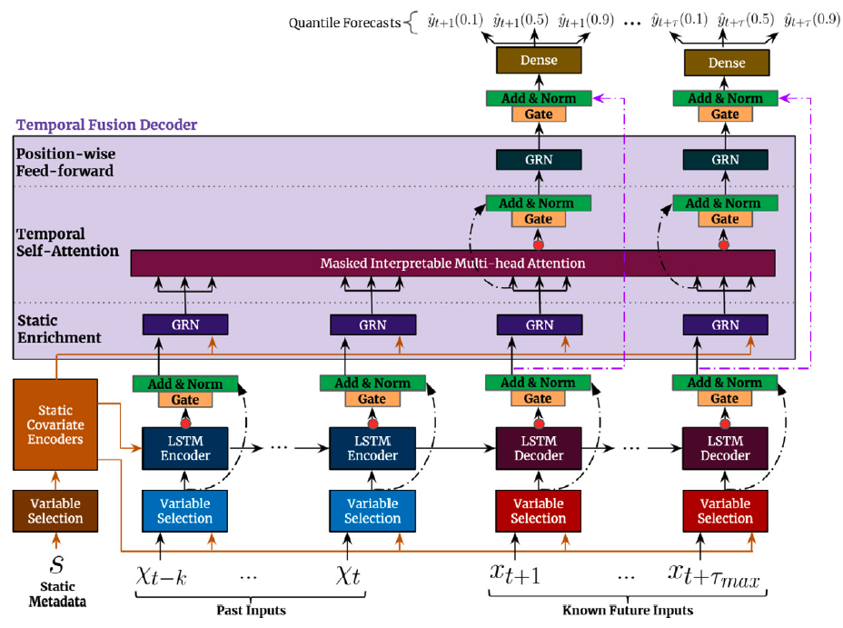 *Figure 1. Temporal Fusion Transformer Architecture.*
## 1. Temporal Fusion Decoder
### `TFT`
```python theme={null}
TFT(
h,
input_size,
tgt_size=1,
stat_exog_list=None,
hist_exog_list=None,
futr_exog_list=None,
hidden_size=128,
n_head=4,
attn_dropout=0.0,
grn_activation="ELU",
n_rnn_layers=1,
rnn_type="lstm",
one_rnn_initial_state=False,
dropout=0.1,
loss=MAE(),
valid_loss=None,
max_steps=1000,
learning_rate=0.001,
num_lr_decays=-1,
early_stop_patience_steps=-1,
val_monitor="ptl/val_loss",
val_check_steps=100,
batch_size=32,
valid_batch_size=None,
windows_batch_size=1024,
inference_windows_batch_size=1024,
start_padding_enabled=False,
training_data_availability_threshold=0.0,
step_size=1,
scaler_type="robust",
random_seed=1,
drop_last_loader=False,
alias=None,
optimizer=None,
optimizer_kwargs=None,
lr_scheduler=None,
lr_scheduler_kwargs=None,
dataloader_kwargs=None,
**trainer_kwargs
)
```
Bases:
*Figure 1. Temporal Fusion Transformer Architecture.*
## 1. Temporal Fusion Decoder
### `TFT`
```python theme={null}
TFT(
h,
input_size,
tgt_size=1,
stat_exog_list=None,
hist_exog_list=None,
futr_exog_list=None,
hidden_size=128,
n_head=4,
attn_dropout=0.0,
grn_activation="ELU",
n_rnn_layers=1,
rnn_type="lstm",
one_rnn_initial_state=False,
dropout=0.1,
loss=MAE(),
valid_loss=None,
max_steps=1000,
learning_rate=0.001,
num_lr_decays=-1,
early_stop_patience_steps=-1,
val_monitor="ptl/val_loss",
val_check_steps=100,
batch_size=32,
valid_batch_size=None,
windows_batch_size=1024,
inference_windows_batch_size=1024,
start_padding_enabled=False,
training_data_availability_threshold=0.0,
step_size=1,
scaler_type="robust",
random_seed=1,
drop_last_loader=False,
alias=None,
optimizer=None,
optimizer_kwargs=None,
lr_scheduler=None,
lr_scheduler_kwargs=None,
dataloader_kwargs=None,
**trainer_kwargs
)
```
Bases: [BaseModel](#neuralforecast.common._base_model.BaseModel)
TFT
The Temporal Fusion Transformer architecture (TFT) is an Sequence-to-Sequence
model that combines static, historic and future available data to predict an
univariate target. The method combines gating layers, an LSTM recurrent encoder,
with and interpretable multi-head attention layer and a multi-step forecasting
strategy decoder.
**Parameters:**
| Name | Type | Description | Default |
| - | - | - | - |
| `h` | [int](#int) | Forecast horizon. | *required* |
| `input_size` | [int](#int) | autorregresive inputs size, y=\[1,2,3,4] input\_size=2 -> y\_\[t-2:t]=\[1,2]. | *required* |
| `tgt_size` | [int](#int) | target size. | 1 |
| `stat_exog_list` | str list | static continuous columns. | None |
| `hist_exog_list` | str list | historic continuous columns. | None |
| `futr_exog_list` | str list | future continuous columns. | None |
| `hidden_size` | [int](#int) | units of embeddings and encoders. | 128 |
| `n_head` | [int](#int) | number of attention heads in temporal fusion decoder. | 4 |
| `attn_dropout` | [float](#float) | dropout of fusion decoder's attention layer. | 0.0 |
| `grn_activation` | [str](#str) | activation for the GRN module from \['ReLU', 'Softplus', 'Tanh', 'SELU', 'LeakyReLU', 'Sigmoid', 'ELU', 'GLU', 'GELU']. | 'ELU' |
| `n_rnn_layers` | [int](#int) | number of RNN layers. | 1 |
| `rnn_type` | [str](#str) | recurrent neural network (RNN) layer type from \["lstm","gru"]. | 'lstm' |
| `one_rnn_initial_state` | [str](#str) | Initialize all rnn layers with the same initial states computed from static covariates. | False |
| `dropout` | [float](#float) | dropout of inputs VSNs. | 0.1 |
| `loss` | PyTorch module | instantiated train loss class from [losses collection](./losses.pytorch.html). | [MAE](#neuralforecast.losses.pytorch.MAE)() |
| `valid_loss` | PyTorch module | instantiated valid loss class from [losses collection](./losses.pytorch.html). | None |
| `max_steps` | [int](#int) | maximum number of training steps. | 1000 |
| `learning_rate` | [float](#float) | Learning rate between (0, 1). | 0.001 |
| `num_lr_decays` | [int](#int) | Number of learning rate decays, evenly distributed across max\_steps. | -1 |
| `early_stop_patience_steps` | [int](#int) | Number of validation iterations before early stopping. | -1 |
| `val_monitor` | [str](#str) | metric to monitor for early stopping. Valid options: "ptl/val\_loss", "valid\_loss", "train\_loss". Default: "ptl/val\_loss". | 'ptl/val\_loss' |
| `val_check_steps` | [int](#int) | Number of training steps between every validation loss check. | 100 |
| `batch_size` | [int](#int) | number of different series in each batch. | 32 |
| `valid_batch_size` | [int](#int) | number of different series in each validation and test batch. | None |
| `windows_batch_size` | [int](#int) | windows sampled from rolled data, default uses all. | 1024 |
| `inference_windows_batch_size` | [int](#int) | number of windows to sample in each inference batch, -1 uses all. | 1024 |
| `start_padding_enabled` | [bool](#bool) | if True, the model will pad the time series with zeros at the beginning, by input size. | False |
| `training_data_availability_threshold` | [Union](#Union)\[[float](#float), [List](#List)\[[float](#float)]] | minimum fraction of valid data points required for training windows. Single float applies to both insample and outsample; list of two floats specifies \[insample\_fraction, outsample\_fraction]. Default 0.0 allows windows with only 1 valid data point (current behavior). | 0.0 |
| `step_size` | [int](#int) | step size between each window of temporal data. | 1 |
| `scaler_type` | [str](#str) | type of scaler for temporal inputs normalization see [temporal scalers](https://github.com/Nixtla/neuralforecast/blob/main/neuralforecast/common/_scalers.py). | 'robust' |
| `random_seed` | [int](#int) | random seed initialization for replicability. | 1 |
| `drop_last_loader` | [bool](#bool) | if True `TimeSeriesDataLoader` drops last non-full batch. | False |
| `alias` | [str](#str) | optional, Custom name of the model. | None |
| `optimizer` | Subclass of 'torch.optim.Optimizer' | optional, user specified optimizer instead of the default choice (Adam). | None |
| `optimizer_kwargs` | [dict](#dict) | optional, list of parameters used by the user specified `optimizer`. | None |
| `lr_scheduler` | Subclass of 'torch.optim.lr\_scheduler.LRScheduler' | optional, user specified lr\_scheduler instead of the default choice (StepLR). | None |
| `lr_scheduler_kwargs` | [dict](#dict) | optional, list of parameters used by the user specified `lr_scheduler`. | None |
| `dataloader_kwargs` | [dict](#dict) | optional, list of parameters passed into the PyTorch Lightning dataloader by the `TimeSeriesDataLoader`. | None |
| `**trainer_kwargs` | [int](#int) | keyword trainer arguments inherited from [PyTorch Lightning's trainer](https://pytorch-lightning.readthedocs.io/en/stable/api/pytorch_lightning.trainer.trainer.Trainer.html?highlight=trainer). | {} |
References
* [Bryan Lim, Sercan O. Arik, Nicolas Loeff, Tomas Pfister, "Temporal Fusion Transformers for interpretable multi-horizon time series forecasting"](https://www.sciencedirect.com/science/article/pii/S0169207021000637)
#### `TFT.fit`
```python theme={null}
fit(
dataset, val_size=0, test_size=0, random_seed=None, distributed_config=None
)
```
Fit.
The `fit` method, optimizes the neural network's weights using the
initialization parameters (`learning_rate`, `windows_batch_size`, ...)
and the `loss` function as defined during the initialization.
Within `fit` we use a PyTorch Lightning `Trainer` that
inherits the initialization's `self.trainer_kwargs`, to customize
its inputs, see [PL's trainer arguments](https://pytorch-lightning.readthedocs.io/en/stable/api/pytorch_lightning.trainer.trainer.Trainer.html?highlight=trainer).
The method is designed to be compatible with SKLearn-like classes
and in particular to be compatible with the StatsForecast library.
By default the `model` is not saving training checkpoints to protect
disk memory, to get them change `enable_checkpointing=True` in `__init__`.
**Parameters:**
| Name | Type | Description | Default |
| - | - | - | - |
| `dataset` | [TimeSeriesDataset](#TimeSeriesDataset) | NeuralForecast's `TimeSeriesDataset`, see [documentation](./tsdataset.html). | *required* |
| `val_size` | [int](#int) | Validation size for temporal cross-validation. | 0 |
| `random_seed` | [int](#int) | Random seed for pytorch initializer and numpy generators, overwrites model.**init**'s. | None |
| `test_size` | [int](#int) | Test size for temporal cross-validation. | 0 |
**Returns:**
| Type | Description |
| - | - |
| None | |
#### `TFT.predict`
```python theme={null}
predict(
dataset,
test_size=None,
step_size=1,
random_seed=None,
quantiles=None,
h=None,
explainer_config=None,
**data_module_kwargs
)
```
Predict.
Neural network prediction with PL's `Trainer` execution of `predict_step`.
**Parameters:**
| Name | Type | Description | Default |
| - | - | - | - |
| `dataset` | [TimeSeriesDataset](#TimeSeriesDataset) | NeuralForecast's `TimeSeriesDataset`, see [documentation](./tsdataset.html). | *required* |
| `test_size` | [int](#int) | Test size for temporal cross-validation. | None |
| `step_size` | [int](#int) | Step size between each window. | 1 |
| `random_seed` | [int](#int) | Random seed for pytorch initializer and numpy generators, overwrites model.**init**'s. | None |
| `quantiles` | [list](#list) | Target quantiles to predict. | None |
| `h` | [int](#int) | Prediction horizon, if None, uses the model's fitted horizon. Defaults to None. | None |
| `explainer_config` | [dict](#dict) | configuration for explanations. | None |
| `**data_module_kwargs` | [dict](#dict) | PL's TimeSeriesDataModule args, see [documentation](https://pytorch-lightning.readthedocs.io/en/1.6.1/extensions/datamodules.html#using-a-datamodule). | {} |
**Returns:**
| Type | Description |
| - | - |
| None | |
#### `TFT.feature_importances`
```python theme={null}
feature_importances()
```
Compute the feature importances for historical, future, and static features.
**Returns:**
| Name | Type | Description |
| - | - | - |
| `dict` | | A dictionary containing the feature importances for each feature type. The keys are 'hist\_vsn', 'future\_vsn', and 'static\_vsn', and the values are pandas DataFrames with the corresponding feature importances. |
#### `TFT.attention_weights`
```python theme={null}
attention_weights()
```
Batch average attention weights
Returns:
np.ndarray: A 1D array containing the attention weights for each time step.
#### `TFT.feature_importance_correlations`
```python theme={null}
feature_importance_correlations()
```
Compute the correlation between the past and future feature importances and the mean attention weights.
Returns:
pd.DataFrame: A DataFrame containing the correlation coefficients between the past feature importances and the mean attention weights.
### Usage Example
```python theme={null}
import matplotlib.pyplot as plt
import numpy as np
import pandas as pd
from neuralforecast import NeuralForecast
# from neuralforecast.models import TFT
from neuralforecast.losses.pytorch import DistributionLoss
from neuralforecast.utils import AirPassengersPanel, AirPassengersStatic
AirPassengersPanel["month"] = AirPassengersPanel.ds.dt.month
Y_train_df = AirPassengersPanel[
AirPassengersPanel.ds < AirPassengersPanel["ds"].values[-12]
] # 132 train
Y_test_df = AirPassengersPanel[
AirPassengersPanel.ds >= AirPassengersPanel["ds"].values[-12]
].reset_index(drop=True) # 12 test
nf = NeuralForecast(
models=[
TFT(
h=12,
input_size=48,
hidden_size=20,
grn_activation="ELU",
rnn_type="lstm",
n_rnn_layers=1,
one_rnn_initial_state=False,
loss=DistributionLoss(distribution="StudentT", level=[80, 90]),
learning_rate=0.005,
stat_exog_list=["airline1"],
futr_exog_list=["y_[lag12]", "month"],
hist_exog_list=["trend"],
max_steps=300,
val_check_steps=10,
early_stop_patience_steps=10,
scaler_type="robust",
windows_batch_size=None,
enable_progress_bar=True,
),
],
freq="ME",
)
nf.fit(df=Y_train_df, static_df=AirPassengersStatic, val_size=12)
Y_hat_df = nf.predict(futr_df=Y_test_df)
# Plot quantile predictions
Y_hat_df = Y_hat_df.reset_index(drop=False).drop(columns=["unique_id", "ds"])
plot_df = pd.concat([Y_test_df, Y_hat_df], axis=1)
plot_df = pd.concat([Y_train_df, plot_df])
plot_df = plot_df[plot_df.unique_id == "Airline1"].drop("unique_id", axis=1)
plt.plot(plot_df["ds"], plot_df["y"], c="black", label="True")
plt.plot(plot_df["ds"], plot_df["TFT"], c="purple", label="mean")
plt.plot(plot_df["ds"], plot_df["TFT-median"], c="blue", label="median")
plt.fill_between(
x=plot_df["ds"][-12:],
y1=plot_df["TFT-lo-90"][-12:].values,
y2=plot_df["TFT-hi-90"][-12:].values,
alpha=0.4,
label="level 90",
)
plt.legend()
plt.grid()
plt.plot()
```
## 2. TFT Architecture
The first TFT’s step is embed the original input
$\{\mathbf{x}^{(s)}, \mathbf{x}^{(h)}, \mathbf{x}^{(f)}\}$ into a high
dimensional space
$\{\mathbf{E}^{(s)}, \mathbf{E}^{(h)}, \mathbf{E}^{(f)}\}$, after which
each embedding is gated by a variable selection network (VSN). The
static embedding $\mathbf{E}^{(s)}$ is used as context for variable
selection and as initial condition to the LSTM. Finally the encoded
variables are fed into the multi-head attention decoder.
### 2.1 Static Covariate Encoder
The static embedding $\mathbf{E}^{(s)}$ is transformed by the
StaticCovariateEncoder into contexts $c_{s}, c_{e}, c_{h}, c_{c}$. Where
$c_{s}$ are temporal variable selection contexts, $c_{e}$ are
TemporalFusionDecoder enriching contexts, and $c_{h}, c_{c}$ are LSTM’s
hidden/contexts for the TemporalCovariateEncoder.
### 2.2 Temporal Covariate Encoder
TemporalCovariateEncoder encodes the embeddings
$\mathbf{E}^{(h)}, \mathbf{E}^{(f)}$ and contexts $(c_{h}, c_{c})$ with
an LSTM.
An analogous process is repeated for the future data, with the main
difference that $\mathbf{E}^{(f)}$ contains the future available
information.
### 2.3 Temporal Fusion Decoder
The TemporalFusionDecoder enriches the LSTM’s outputs with $c_{e}$ and
then uses an attention layer, and multi-step adapter.
## 3. Interpretability
### 3.1 Attention Weights
```python theme={null}
attention = nf.models[0].attention_weights()
```
```python theme={null}
def plot_attention(
self, plot: str = "time", output: str = "plot", width: int = 800, height: int = 400
):
"""
Plot the attention weights.
Args:
plot (str, optional): The type of plot to generate. Can be one of the following:
- 'time': Display the mean attention weights over time.
- 'all': Display the attention weights for each horizon.
- 'heatmap': Display the attention weights as a heatmap.
- An integer in the range [1, model.h) to display the attention weights for a specific horizon.
output (str, optional): The type of output to generate. Can be one of the following:
- 'plot': Display the plot directly.
- 'figure': Return the plot as a figure object.
width (int, optional): Width of the plot in pixels. Default is 800.
height (int, optional): Height of the plot in pixels. Default is 400.
Returns:
matplotlib.figure.Figure: If `output` is 'figure', the function returns the plot as a figure object.
"""
attention = (
self.mean_on_batch(self.interpretability_params["attn_wts"])
.mean(dim=0)
.cpu()
.numpy()
)
fig, ax = plt.subplots(figsize=(width / 100, height / 100))
if plot == "time":
attention = attention[self.input_size :, :].mean(axis=0)
ax.plot(np.arange(-self.input_size, self.h), attention)
ax.axvline(
x=0, color="black", linewidth=3, linestyle="--", label="prediction start"
)
ax.set_title("Mean Attention")
ax.set_xlabel("time")
ax.set_ylabel("Attention")
ax.legend()
elif plot == "all":
for i in range(self.input_size, attention.shape[0]):
ax.plot(
np.arange(-self.input_size, self.h),
attention[i, :],
label=f"horizon {i-self.input_size+1}",
)
ax.axvline(
x=0, color="black", linewidth=3, linestyle="--", label="prediction start"
)
ax.set_title("Attention per horizon")
ax.set_xlabel("time")
ax.set_ylabel("Attention")
ax.legend()
elif plot == "heatmap":
cax = ax.imshow(
attention,
aspect="auto",
cmap="viridis",
extent=[-self.input_size, self.h, -self.input_size, self.h],
)
fig.colorbar(cax)
ax.set_title("Attention Heatmap")
ax.set_xlabel("Attention (current time step)")
ax.set_ylabel("Attention (previous time step)")
elif isinstance(plot, int) and (plot in np.arange(1, self.h + 1)):
i = self.input_size + plot - 1
ax.plot(
np.arange(-self.input_size, self.h),
attention[i, :],
label=f"horizon {plot}",
)
ax.axvline(
x=0, color="black", linewidth=3, linestyle="--", label="prediction start"
)
ax.set_title(f"Attention weight for horizon {plot}")
ax.set_xlabel("time")
ax.set_ylabel("Attention")
ax.legend()
else:
raise ValueError(
'plot has to be in ["time","all","heatmap"] or integer in range(1,model.h)'
)
plt.tight_layout()
if output == "plot":
plt.show()
elif output == "figure":
return fig
else:
raise ValueError(f"Invalid output: {output}. Expected 'plot' or 'figure'.")
```
##### 3.1.1 Mean attention
```python theme={null}
plot_attention(nf.models[0], plot="time")
```
##### 3.1.2 Attention of all future time steps
```python theme={null}
plot_attention(nf.models[0], plot="all")
```
##### 3.1.3 Attention of a specific future time step
```python theme={null}
plot_attention(nf.models[0], plot=8)
```
### 3.2 Feature Importance
#### 3.2.1 Global feature importance
```python theme={null}
feature_importances = nf.models[0].feature_importances()
feature_importances.keys()
```
##### Static variable importances
```python theme={null}
feature_importances["Static covariates"].sort_values(by="importance").plot(kind="barh")
```
##### Past variable importances
```python theme={null}
feature_importances["Past variable importance over time"].mean().sort_values().plot(
kind="barh"
)
```
##### Future variable importances
```python theme={null}
feature_importances["Future variable importance over time"].mean().sort_values().plot(
kind="barh"
)
```
#### 3.2.2 Variable importances over time
##### Future variable importance over time
Importance of each future covariate at each future time step
```python theme={null}
df = feature_importances["Future variable importance over time"]
fig, ax = plt.subplots(figsize=(20, 10))
bottom = np.zeros(len(df.index))
for col in df.columns:
p = ax.bar(np.arange(-len(df), 0), df[col].values, 0.6, label=col, bottom=bottom)
bottom += df[col]
ax.set_title("Future variable importance over time ponderated by attention")
ax.set_ylabel("Importance")
ax.set_xlabel("Time")
ax.grid(True)
ax.legend()
plt.show()
```
##### Past variable importance over time
```python theme={null}
df = feature_importances["Past variable importance over time"]
fig, ax = plt.subplots(figsize=(20, 10))
bottom = np.zeros(len(df.index))
for col in df.columns:
p = ax.bar(np.arange(-len(df), 0), df[col].values, 0.6, label=col, bottom=bottom)
bottom += df[col]
ax.set_title("Past variable importance over time")
ax.set_ylabel("Importance")
ax.set_xlabel("Time")
ax.legend()
ax.grid(True)
plt.show()
```
##### Past variable importance over time ponderated by attention
Decomposition of the importance of each time step based on importance of
each variable at that time step
```python theme={null}
df = feature_importances["Past variable importance over time"]
mean_attention = (
nf.models[0]
.attention_weights()[nf.models[0].input_size :, :]
.mean(axis=0)[: nf.models[0].input_size]
)
df = df.multiply(mean_attention, axis=0)
fig, ax = plt.subplots(figsize=(20, 10))
bottom = np.zeros(len(df.index))
for col in df.columns:
p = ax.bar(np.arange(-len(df), 0), df[col].values, 0.6, label=col, bottom=bottom)
bottom += df[col]
ax.set_title("Past variable importance over time ponderated by attention")
ax.set_ylabel("Importance")
ax.set_xlabel("Time")
ax.legend()
ax.grid(True)
plt.plot(
np.arange(-len(df), 0),
mean_attention,
color="black",
marker="o",
linestyle="-",
linewidth=2,
label="mean_attention",
)
plt.legend()
plt.show()
```
#### 3.2.3 Variable importance correlations over time
Variables which gain and lose importance at same moments
```python theme={null}
nf.models[0].feature_importance_correlations()
```
## 4. Auxiliary Functions
### 4.1 Gating Mechanisms
The Gated Residual Network (GRN) provides adaptive depth and network
complexity capable of accommodating different size datasets. As residual
connections allow for the network to skip the non-linear transformation
of input $\mathbf{a}$ and context $\mathbf{c}$.
The Gated Linear Unit (GLU) provides the flexibility of suppressing
unnecessary parts of the GRN. Consider GRN’s output $\gamma$ then GLU
transformation is defined by:
$\mathrm{GLU}(\gamma) = \sigma(\mathbf{W}_{4}\gamma +b_{4}) \odot (\mathbf{W}_{5}\gamma +b_{5})$
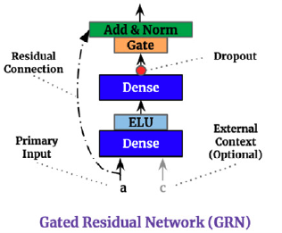 *Figure 2. Gated Residual Network.*
### 4.2 Variable Selection Networks
TFT includes automated variable selection capabilities, through its
variable selection network (VSN) components. The VSN takes the original
input
$\{\mathbf{x}^{(s)}, \mathbf{x}^{(h)}_{[:t]}, \mathbf{x}^{(f)}_{[:t]}\}$
and transforms it through embeddings or linear transformations into a
high dimensional space
$\{\mathbf{E}^{(s)}, \mathbf{E}^{(h)}_{[:t]}, \mathbf{E}^{(f)}_{[:t+H]}\}$.
For the observed historic data, the embedding matrix
$\mathbf{E}^{(h)}_{t}$ at time $t$ is a concatenation of $j$ variable
$e^{(h)}_{t,j}$ embeddings:
The variable selection weights are given by:
$s^{(h)}_{t}=\mathrm{SoftMax}(\mathrm{GRN}(\mathbf{E}^{(h)}_{t},\mathbf{E}^{(s)}))$
The VSN processed features are then:
$\tilde{\mathbf{E}}^{(h)}_{t}= \sum_{j} s^{(h)}_{j} \tilde{e}^{(h)}_{t,j}$
*Figure 2. Gated Residual Network.*
### 4.2 Variable Selection Networks
TFT includes automated variable selection capabilities, through its
variable selection network (VSN) components. The VSN takes the original
input
$\{\mathbf{x}^{(s)}, \mathbf{x}^{(h)}_{[:t]}, \mathbf{x}^{(f)}_{[:t]}\}$
and transforms it through embeddings or linear transformations into a
high dimensional space
$\{\mathbf{E}^{(s)}, \mathbf{E}^{(h)}_{[:t]}, \mathbf{E}^{(f)}_{[:t+H]}\}$.
For the observed historic data, the embedding matrix
$\mathbf{E}^{(h)}_{t}$ at time $t$ is a concatenation of $j$ variable
$e^{(h)}_{t,j}$ embeddings:
The variable selection weights are given by:
$s^{(h)}_{t}=\mathrm{SoftMax}(\mathrm{GRN}(\mathbf{E}^{(h)}_{t},\mathbf{E}^{(s)}))$
The VSN processed features are then:
$\tilde{\mathbf{E}}^{(h)}_{t}= \sum_{j} s^{(h)}_{j} \tilde{e}^{(h)}_{t,j}$
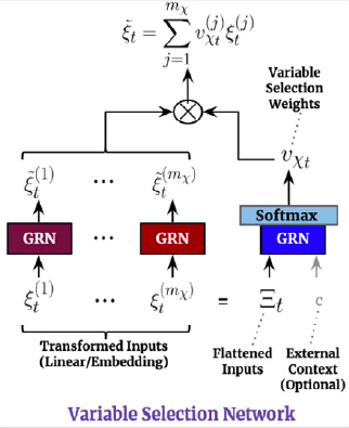 *Figure 3. Variable Selection Network*
### 4.3. Multi-Head Attention
To avoid information bottlenecks from the classic Seq2Seq architecture,
TFT incorporates a decoder-encoder attention mechanism inherited
transformer architectures ([Li et. al
2019](https://arxiv.org/abs/1907.00235), [Vaswani et. al
2017](https://arxiv.org/abs/1706.03762)). It transforms the outputs
of the LSTM encoded temporal features, and helps the decoder better
capture long-term relationships.
The original multihead attention for each component $H_{m}$ and its
query, key, and value representations are denoted by
$Q_{m}, K_{m}, V_{m}$, its transformation is given by:
TFT modifies the original multihead attention to improve its
interpretability. To do it it uses shared values $\tilde{V}$ across
heads and employs additive aggregation,
$\mathrm{InterpretableMultiHead}(Q,K,V) = \tilde{H} W_{M}$. The
mechanism has a great resemblence to a single attention layer, but it
allows for $M$ multiple attention weights, and can be therefore be
interpreted as the average ensemble of $M$ single attention layers.
## Related topics
- [Forecasting with TFT: Temporal Fusion Transformer](/neuralforecast/docs/tutorials/forecasting_tft.html.md)
- [iTransformer Time Series Forecasting in Python](/neuralforecast/models.itransformer.html.md)
- [Informer Time Series Forecasting in Python](/neuralforecast/models.informer.html.md)
- [Automatic Forecasting](/neuralforecast/models.html.md)
- [PatchTST Time Series Forecasting in Python](/neuralforecast/models.patchtst.html.md)
*Figure 3. Variable Selection Network*
### 4.3. Multi-Head Attention
To avoid information bottlenecks from the classic Seq2Seq architecture,
TFT incorporates a decoder-encoder attention mechanism inherited
transformer architectures ([Li et. al
2019](https://arxiv.org/abs/1907.00235), [Vaswani et. al
2017](https://arxiv.org/abs/1706.03762)). It transforms the outputs
of the LSTM encoded temporal features, and helps the decoder better
capture long-term relationships.
The original multihead attention for each component $H_{m}$ and its
query, key, and value representations are denoted by
$Q_{m}, K_{m}, V_{m}$, its transformation is given by:
TFT modifies the original multihead attention to improve its
interpretability. To do it it uses shared values $\tilde{V}$ across
heads and employs additive aggregation,
$\mathrm{InterpretableMultiHead}(Q,K,V) = \tilde{H} W_{M}$. The
mechanism has a great resemblence to a single attention layer, but it
allows for $M$ multiple attention weights, and can be therefore be
interpreted as the average ensemble of $M$ single attention layers.
## Related topics
- [Forecasting with TFT: Temporal Fusion Transformer](/neuralforecast/docs/tutorials/forecasting_tft.html.md)
- [iTransformer Time Series Forecasting in Python](/neuralforecast/models.itransformer.html.md)
- [Informer Time Series Forecasting in Python](/neuralforecast/models.informer.html.md)
- [Automatic Forecasting](/neuralforecast/models.html.md)
- [PatchTST Time Series Forecasting in Python](/neuralforecast/models.patchtst.html.md)